Glow 0.4 Enables Integration of Genomic Variant and Annotation Data
Glow 0.4 was released on May 20, 2020. This blog focuses on the highlight of this release, the newly introduced capability to ingest genomic annotation data from the GFF3 (Generic Feature Format Version 3) flat file format. This release also includes other feature and usability improvements, which will be briefly reviewed at the end of this blog.
GFF3 is a sequence annotation flat file format proposed by the Sequence Ontology Project in 2013, which since has become the de facto format for genome annotation and is widely used by genome browsers and databases such as NCBI RefSeq and GenBank. GFF3, a 9-column tab-separated text format, typically carries the majority of the annotation data in the ninth column, called attributes, as a semi-colon-separated list of <tag>=<value> entries. As a result, although GFF3 files can be read as Spark DataFrames using Spark SQL’s standard csv data source, the schema of the resulting DataFrame would be quite unwieldy for query and data manipulation of annotation data, because the whole list of attribute tag-value pairs for each sequence will appear as a single semi-colon-separated string in the attributes column of the DataFrame.
Glow 0.4 adds the new and flexible gff Spark SQL data source to address this challenge and create a smooth GFF3 ingest and query experience. While reading the GFF3 file, the gff data source parses the attributes column of the file to create an appropriately typed column for each tag. In each row, this column will contain the value corresponding to that tag in that row (or null if the tag does not appear in the row). Consequently, all tags in the GFF3 attributes column will have their own corresponding column in the Spark DataFrame, making annotation data query and manipulation much easier.
Ingesting GFF3 Annotation Data
Like any other Spark data source, reading GFF3 files using Glow’s gff data source can be done in a single line of code. As an example, we can ingest the annotations of the Homo Sapiens genome assembly GRCh38.p13 from a GFF3 file. Here, we have also filtered the annotations to chromosome 22 in order to use the resulting annotations_df DataFrame (Fig. 6) in continuation of our example. The annotations_df alias is for the same purpose as well.
import glow
spark = glow.register(spark)

gff_path = '/databricks-datasets/genomics/gffs/GCF_000001405.39_GRCh38.p13_genomic.gff.bgz'

annotations_df = spark.read.format('gff').load(gff_path) \
    .filter("seqid = 'NC_000022.11'") \
    .alias('annotations_df')
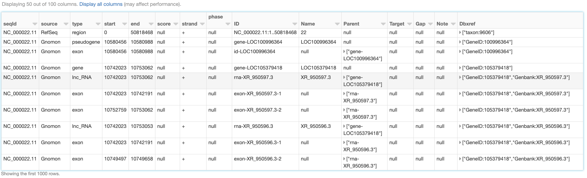
Fig. 6 A small section of the annotations_df DataFrame
In addition to reading uncompressed .gff files, the gff data source supports all compression formats supported by Spark’s csv data source, including .gz and .bgz. It is strongly recommended to use splittable compression formats like .bgz instead of .gz for better parallelization of the read process.
Schema
Let us have a closer look at the schema of the resulting DataFrame, which was automatically inferred by Glow’s gff data source:
annotations_df.printSchema()
root
 |-- seqId: string (nullable = true)
 |-- source: string (nullable = true)
 |-- type: string (nullable = true)
 |-- start: long (nullable = true)
 |-- end: long (nullable = true)
 |-- score: double (nullable = true)
 |-- strand: string (nullable = true)
 |-- phase: integer (nullable = true)
 |-- ID: string (nullable = true)
 |-- Name: string (nullable = true)
 |-- Parent: array (nullable = true)
 |    |-- element: string (containsNull = true)
 |-- Target: string (nullable = true)
 |-- Gap: string (nullable = true)
 |-- Note: array (nullable = true)
 |    |-- element: string (containsNull = true)
 |-- Dbxref: array (nullable = true)
 |    |-- element: string (containsNull = true)
 |-- Is_circular: boolean (nullable = true)
 |-- align_id: string (nullable = true)
 |-- allele: string (nullable = true)
 .
 .
 .
 |-- transl_table: string (nullable = true)
 |-- weighted_identity: string (nullable = true)
This schema has 100 fields (not all shown here). The first eight fields (seqId, source, type, start, end, score, strand, and phase), here referred to as the “base” fields, correspond to the first eight columns of the GFF3 format cast in the proper data types. The rest of the fields in the inferred schema are the result of parsing the attributes column of the GFF3 file. Fields corresponding to any “official” tag (those referred to as “tags with pre-defined meaning” in the GFF3 format description), if present in the GFF3 file, come first in appropriate data types. The official fields are followed by the “unofficial” fields (fields corresponding to any other tag) in alphabetical order. In the example above, ID, Name, Parent, Target, Gap, Note, Dbxref, and Is_circular are the official fields, and the rest are the unofficial fields. The gff data source discards the comments, directives, and FASTA lines that may be in the GFF3 file.
As it is not uncommon for the official tags to be spelled differently in terms of letter case and underscore usage across different GFF3 files, or even within a single GFF3 file, the gff data source is designed to be insensitive to letter case and underscore in extracting official tags from the attributes field. For example, the official tag Dbxref will be correctly extracted as an official field even if it appears as dbxref or dbx_ref in the GFF3 file. Please see Glow documentation for more details.
Like other Spark SQL data sources, Glow’s gff data source is also able to accept a user-specified schema through the .schema command. The data source behavior in this case is also designed to be quite flexible. More specifically, the fields (and their types) in the user-specified schema are treated as the list of fields, whether base, official, or unofficial, to be extracted from the GFF3 file (and cast to the specified types). Please see the Glow documentation for more details on how user-specified schemas can be used.
Example: Gene Transcripts and Transcript Exons
With the annotation tags extracted as individual DataFrame columns using Glow’s gff data source, query and data preparation over genetic annotations becomes as easy as writing common Spark SQL commands in the user’s API of choice. As an example, here we demonstrate how simple queries can be used to extract data regarding hierarchical grouping of genomic features from the annotations_df created above.
One of the main advantages of the GFF3 format compared to older versions of GFF is the improved presentation of feature hierarchies (see GFF3 format description for more details). Two examples of such hierarchies are:
Transcripts of a gene (here, gene is the “parent” feature and its transcripts are the “children” features).
Exons of a transcript (here, the transcript is the parent and its exons are the children).
In the GFF3 format, the parents of the feature in each row are identified by the value of the parent tag in the attributes column, which includes the ID(s) of the parent(s) of the row. Glow’s gff data source extracts this information as an array of parent ID(s) in a column of the resulting DataFrame called parent.
Assume we would like to create a DataFrame, called gene_transcript_df, which, for each gene on chromosome 22, provides some basic information about the gene and all its transcripts. As each row in the annotations_df of our example has at most a single parent, the parent_child_df DataFrame created by the following query will help us in achieving our goal. This query joins annotations_df with a subset of its own columns on the parent column as the key. Fig. 7 shows a small section of parent_child_df.
from pyspark.sql.functions import *

parent_child_df = annotations_df \
.join(
  annotations_df.select('id', 'type', 'name', 'start', 'end').alias('parent_df'),
  col('annotations_df.parent')[0] == col('parent_df.id') # each row in annotation_df has at most one parent
) \
.orderBy('annotations_df.start', 'annotations_df.end') \
.select(
  'annotations_df.seqid',
  'annotations_df.type',
  'annotations_df.start',
  'annotations_df.end',
  'annotations_df.id',
  'annotations_df.name',
  col('annotations_df.parent')[0].alias('parent_id'),
  col('parent_df.Name').alias('parent_name'),
  col('parent_df.type').alias('parent_type'),
  col('parent_df.start').alias('parent_start'),
  col('parent_df.end').alias('parent_end')
) \
.alias('parent_child_df')
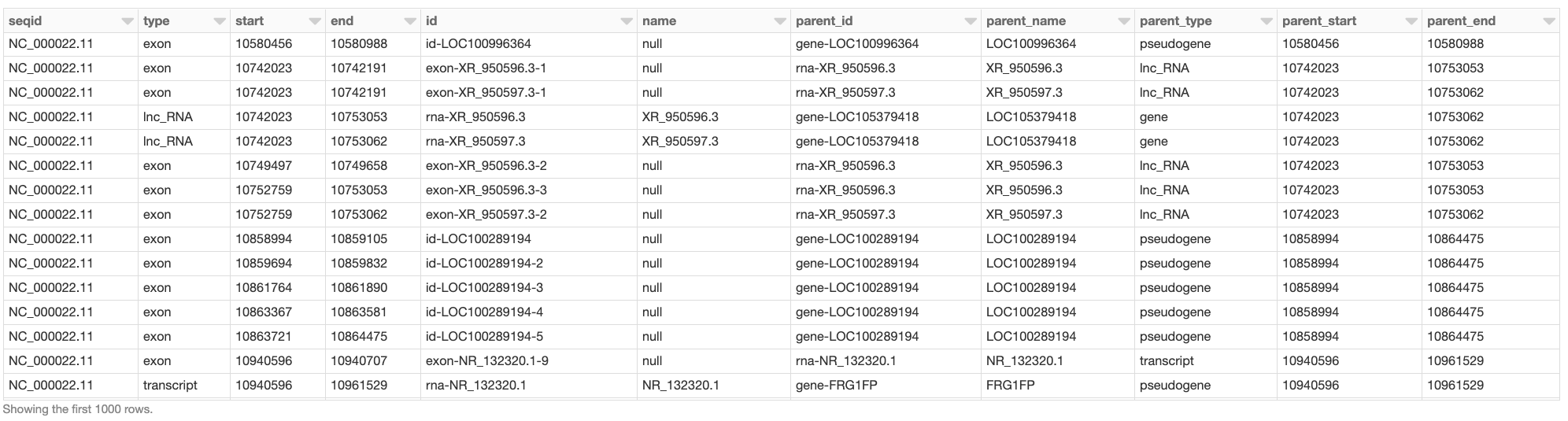
Fig. 7 A small section of the parent_child_df DataFrame
Having the parent_child_df DataFrame, we can now write the following simple function, called parent_child_summary, which, given this DataFrame, the parent type, and the child type, generates a DataFrame containing basic information on each parent of the given type and all its children of the given type.
from pyspark.sql.dataframe import *

def parent_child_summary(parent_child_df: DataFrame, parent_type: str, child_type: str) -> DataFrame:
  return parent_child_df \
    .select(
      'seqid',
      col('parent_id').alias(f'{parent_type}_id'),
      col('parent_name').alias(f'{parent_type}_name'),
      col('parent_start').alias(f'{parent_type}_start'),
      col('parent_end').alias(f'{parent_type}_end'),
      col('id').alias(f'{child_type}_id'),
      col('start').alias(f'{child_type}_start'),
      col('end').alias(f'{child_type}_end'),
    ) \
    .where(f"type == '{child_type}' and parent_type == '{parent_type}'") \
    .groupBy(
      'seqid',
      f'{parent_type}_id',
      f'{parent_type}_name',
      f'{parent_type}_start',
      f'{parent_type}_end'
    ) \
    .agg(
      collect_list(
        struct(
          f'{child_type}_id',
          f'{child_type}_start',
          f'{child_type}_end'
        )
      ).alias(f'{child_type}s')
    ) \
    .orderBy(
      f'{parent_type}_start',
      f'{parent_type}_end'
    ) \
    .alias(f'{parent_type}_{child_type}_df')
Now we can generate our intended gene_transcript_df DataFrame, shown in Fig. 8, with a single call to this function:
gene_transcript_df = parent_child_summary(parent_child_df, 'gene', 'transcript')
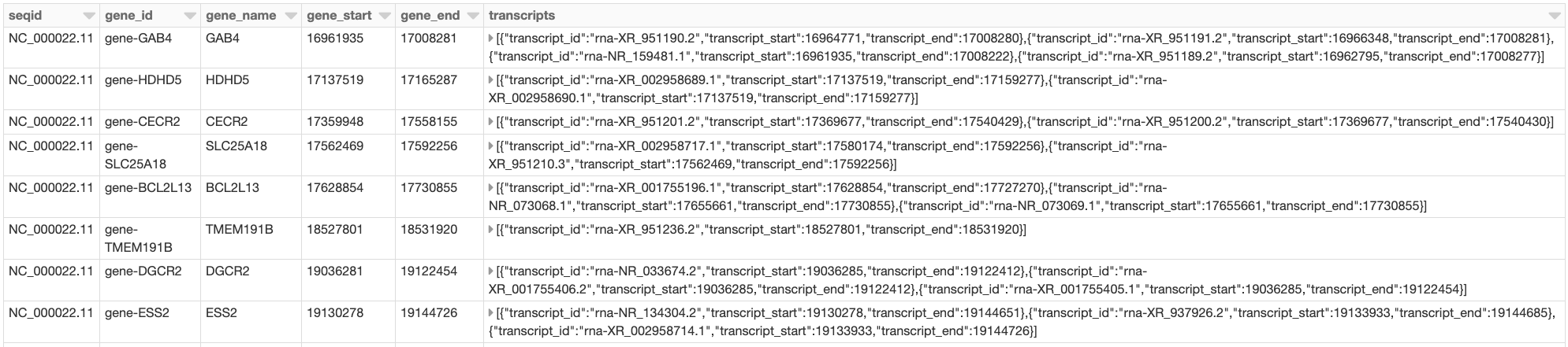
Fig. 8 A small section of the gene_transcript_df DataFrame
In each row of this DataFrame, the transcripts column contains the ID, start and end of all transcripts of the gene in that row as an array of structs.
The same function can now be used to generate any parent-child feature summary. For example, we can generate the information of all exons of each transcript on chromosome 22 with another call to the parent_child_summary function as shown below. Fig. 9 shows the generated transcript_exon_df DataFrame.
transcript_exon_df = parent_child_summary(parent_child_df, 'transcript', 'exon')
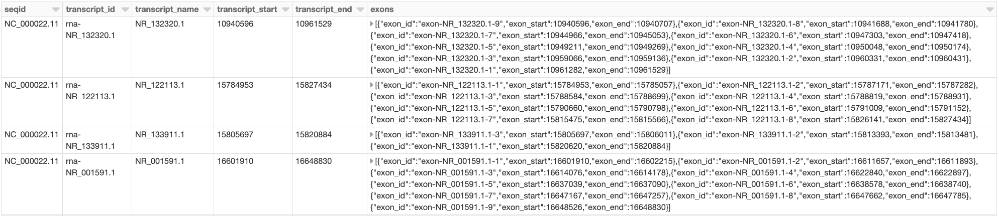
Fig. 9 A small section of the transcript_exon_df DataFrame
Example Continued: Integration with Variant Data
Glow has data sources to ingest variant data from common flat file formats such as VCF, BGEN, and PLINK. Combining the power of Glow’s variant data sources with the new gff data source, the users can now seamlessly annotate their variant DataFrames by joining them with annotation DataFrames in any desired fashion.
As an example, let us load the chromosome 22 variants of the 1000 Genome Project (on genome assembly GRCh38) from a VCF file (obtained from the project’s ftp site). Fig. 10 shows the resulting variants_df.
vcf_path = "/databricks-datasets/genomics/1kg-vcfs/ALL.chr22.shapeit2_integrated_snvindels_v2a_27022019.GRCh38.phased.vcf.gz"

variants_df = spark.read \
  .format("vcf") \
  .load(vcf_path) \
  .alias('variants_df')
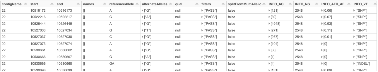
Fig. 10 A small section of the variants_df DataFrame
Now using the following double-join query, we can create a DataFrame which, for each variant on a gene on chromosome 22, provides the information of the variant as well as the exon, transcript, and gene on which the variant resides (Fig. 11). Note that the first two exploded DataFrames can also be constructed directly from parent_child_df. Here, since we had already defined gene_transcrip_df and transcript_exon_df, we generated these exploded DataFrames simply by applying the explode function followed by Glow’s expand_struct function on them.
from glow.functions import *

gene_transcript_exploded_df = gene_transcript_df \
  .withColumn('transcripts', explode('transcripts')) \
  .withColumn('transcripts', expand_struct('transcripts')) \
  .alias('gene_transcript_exploded_df')

transcript_exon_exploded_df = transcript_exon_df \
  .withColumn('exons', explode('exons')) \
  .withColumn('exons', expand_struct('exons')) \
  .alias('transcript_exon_exploded_df')

variant_exon_transcript_gene_df = variants_df \
.join(
  transcript_exon_exploded_df,
  (variants_df.start < transcript_exon_exploded_df.exon_end) &
  (transcript_exon_exploded_df.exon_start < variants_df.end)
) \
.join(
  gene_transcript_exploded_df,
  transcript_exon_exploded_df.transcript_id == gene_transcript_exploded_df.transcript_id
) \
.select(
  col('variants_df.contigName').alias('variant_contig'),
  col('variants_df.start').alias('variant_start'),
  col('variants_df.end').alias('variant_end'),
  col('variants_df.referenceAllele'),
  col('variants_df.alternateAlleles'),
  'transcript_exon_exploded_df.exon_id',
  'transcript_exon_exploded_df.exon_start',
  'transcript_exon_exploded_df.exon_end',
  'transcript_exon_exploded_df.transcript_id',
  'transcript_exon_exploded_df.transcript_name',
  'transcript_exon_exploded_df.transcript_start',
  'transcript_exon_exploded_df.transcript_end',
  'gene_transcript_exploded_df.gene_id',
  'gene_transcript_exploded_df.gene_name',
  'gene_transcript_exploded_df.gene_start',
  'gene_transcript_exploded_df.gene_end'
) \
.orderBy(
  'variant_contig',
  'variant_start',
  'variant_end'
)
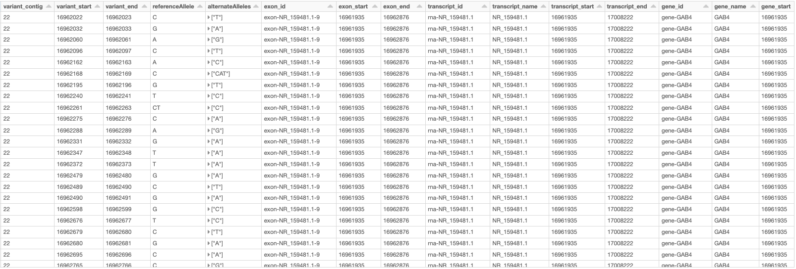
Fig. 11 A small section of the variant_exon_transcript_gene_df DataFrame
Other Features and Improvements
In addition to the new gff reader, Glow 0.4 introduced other features and improvements. A new function, called mean_substitute, was introduced, which can be used to substitute the missing values of a numeric Spark array with the mean of the non-missing values. The normalize_variants transformer now accepts reference genomes in bgzipped fasta format in addition to the uncompressed fasta. The VCF reader was updated to be able to handle reading file globs that include tabix index files. In addition, this reader no longer has the splitToBiallelic option. The split_multiallelics transformer introduced in Glow 0.3 can be used instead. Also, the pipe transformer was improved so that it does not pipe empty partitions. As a result, users do not need to repartition or coalesce when piping VCF files. For a complete list of new features and improvements in Glow 0.4, please refer to Glow 0.4 Release Notes.
Try It!
Try Glow 0.4 and its new features here.