GloWGR: Whole Genome Regression
Glow supports Whole Genome Regression (WGR) as GloWGR, a distributed version of the regenie method (see the paper published in Nature Genetics). GloWGR supports two types of phenotypes:
Quantitative
Binary
Many steps of the GloWGR workflow explained in this page are common between the two cases. Any step that is different between the two has separate explanations clearly marked by “for quantitative phenotypes” vs. “for binary phenotypes”.
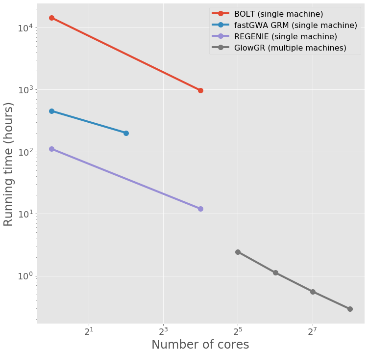
Performance
The following figure demonstrates the performance gain obtained by using parallelized GloWGR in comparision with single machine BOLT, fastGWA GRM, and regenie for fitting WGR models against 50 quantitative phenotypes from the UK Biobank project.
Overview
GloWGR consists of the following stages:
Block the genotype matrix across samples and variants
Perform dimensionality reduction with linear ridge regression
Estimate phenotypic predictors using
For quantitative phenotypes: linear ridge regression
For binary phenotypes: logistic ridge regression
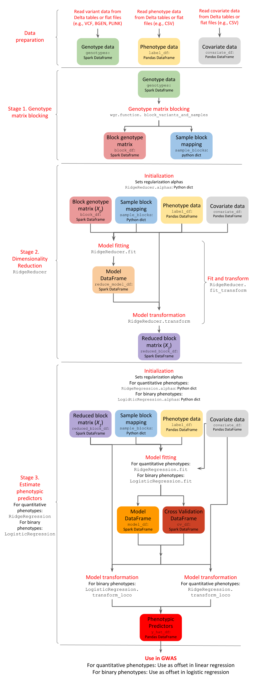
The following diagram provides an overview of the operations and data within the stages of GlowWGR and their interrelationship.
Data preparation
GloWGR accepts three input data components.
1. Genotype data
The genotype data may be read as a Spark DataFrame from any variant data source supported by Glow, such as VCF, BGEN or PLINK. For scalability and high-performance repeated use, we recommend storing flat genotype files into Delta tables.
The DataFrame must include a column values containing a numeric representation of each genotype. The genotypic values may not be missing.
When loading the variants into the DataFrame, perform the following transformations:
Split multiallelic variants with the
split_multiallelicstransformer.Create a
valuescolumn by calculating the numeric representation of each genotype. This representation is typically the number of alternate alleles for biallelic variants which can be calculated withglow.genotype_states. Replace any missing values with the mean of the non-missing values usingglow.mean_substitute.
Example
from pyspark.sql.functions import col, lit

variants = spark.read.format('vcf').load(genotypes_vcf)
genotypes = variants.withColumn('values', glow.mean_substitute(glow.genotype_states(col('genotypes'))))
2. Phenotype data
The phenotype data is represented as a Pandas DataFrame indexed by the sample ID. Phenotypes are also referred to as labels. Each column represents a single phenotype. It is assumed that there are no missing phenotype values. There is no need to standardize the phenotypes. GloWGR automatically standardizes the data before usage if necessary.
For quantitative phenotypes:
import pandas as pd
label_df = pd.read_csv(continuous_phenotypes_csv, index_col='sample_id')[['Continuous_Trait_1', 'Continuous_Trait_2']]
For binary phenotypes: Phenotype values are either 0 or 1.
Example
import pandas as pd
label_df = pd.read_csv(binary_phenotypes_csv, index_col='sample_id')
3. Covariate data
The covariate data is represented as a Pandas DataFrame indexed by the sample ID. Each column represents a single covariate. It is assumed that there are no missing covariate values. There is no need to standardize the covariates. GloWGR automatically standardizes the data before usage if necessary.
Example
covariate_df = pd.read_csv(covariates_csv, index_col='sample_id')
Stage 1. Genotype matrix blocking
The first stage of GloWGR is to generate the block genotype matrix. The glow.wgr.functions.block_variants_and_samples function is used for this purpose and creates two objects: a block genotype matrix and a sample block mapping.
Warning
We do not recommend using the split_multiallelics transformer and the block_variants_and_samples function
in the same query due to JVM JIT code size limits during whole-stage code generation. It is best to persist the
variants after splitting multiallelics to a Delta table (see Create a Genomics Delta Lake) and then read the data from
this Delta table to apply block_variants_and_samples.
Parameters
genotypes: Genotype DataFrame including thevaluescolumn generated as explained abovesample_ids: A python List of sample IDs. Can be created by applyingglow.wgr.functions.get_sample_idsto a genotype DataFramevariants_per_block: Number of variants to include in each block. We recommend 1000.sample_block_count: Number of sample blocks to create. We recommend 10.
Return
The function returns a block genotype matrix and a sample block mapping.
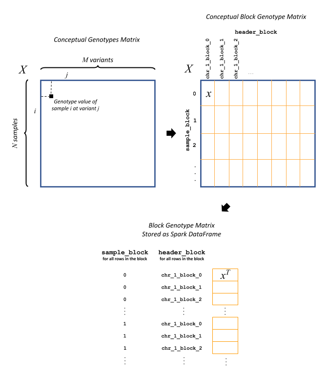
Block genotype matrix (see figure below): The block genotype matrix can be conceptually imagined as an \(N \times M\) matrix \(X\) where each row represents an individual sample, and each column represents a variant, and each cell \((i, j)\) contains the genotype value for sample \(i\) at variant \(j\). Then imagine a coarse grid is laid on top of matrix \(X\) such that matrix cells within the same coarse grid cell are all assigned to the same block. Each block \(x\) is indexed by a sample block ID (corresponding to a list of rows belonging to the block) and a header block ID (corresponding to a list of columns belonging to the block). The sample block IDs are generally just integers 0 through the number of sample blocks. The header block IDs are strings of the form ‘chr_C_block_B’, which refers to the Bth block on chromosome C. The Spark DataFrame representing this block matrix can be thought of as the transpose of each block, i.e., \(x^T\), all stacked one atop another. Each row in the DataFrame represents the values from a particular column of \(X\) for the samples corresponding to a particular sample block.
The fields in the DataFrame and their content for a given row are as follows:
sample_block: An ID assigned to the block \(x\) containing the group of samples represented on this row
header_block: An ID assigned to the block \(x\) containing this header
header: The column name in the conceptual genotype matrix \(X\)
size: The number of individuals in the sample block
values: Genotype values for the header in this sample block. If the matrix is sparse, contains only non-zero values.
position: An integer assigned to this header that specifies the correct sort order for the headers in this block
mu: The mean of the genotype values for this header
sig: The standard deviation of the genotype values for this headerWarning
Variant rows in the input DataFrame whose genotype values are uniform across all samples are filtered from the output block genotype matrix.
Sample block mapping: The sample block mapping is a python dictionary containing key-value pairs, where each key is a sample block ID and each value is a list of sample IDs contained in that sample block. The order of these IDs match the order of the
valuesarrays in the block genotype DataFrame.
Example
from glow.wgr import RidgeReduction, RidgeRegression, LogisticRidgeRegression, block_variants_and_samples, get_sample_ids
from pyspark.sql.functions import col, lit

variants_per_block = 1000
sample_block_count = 10
sample_ids = get_sample_ids(genotypes)
block_df, sample_blocks = block_variants_and_samples(
    genotypes, sample_ids, variants_per_block, sample_block_count)
Stage 2. Dimensionality reduction
Having the block genotype matrix, the first stage is to apply a dimensionality reduction to the block matrix \(X\) using the RidgeReduction class. After RidgeReduction is initialized, dimensionality reduction is accomplished within two steps:
Model fitting, performed by the
RidgeReduction.fitfunction, which fits multiple ridge models within each block \(x\).Model transformation, performed by the
RidgeReduction.transformfunction, which produces a new block matrix where each column represents the prediction of one ridge model applied within one block.
This approach to model building is generally referred to as stacking. We call the starting block genotype matrix the level 0 matrix in the stack, denoted by \(X_0\), and the output of the ridge reduction step the level 1 matrix, denoted by \(X_1\). As one of its initialization, the RidgeReduction class generates (or receives) a list of ridge regularization values (here referred to as alpha). Since ridge models are indexed by these alpha values, RidgeReduction will generate one ridge model per value of alpha provided, which in turn will produce one column per block in \(X_0\). Therefore, the final dimensions of \(X_1\) for a single phenotype will be \(N \times (L \times K)\), where \(L\) is the number of header blocks in \(X_0\) and \(K\) is the number of alpha values provided to RidgeReduction. In practice, we can estimate a span of alpha values in a reasonable order of magnitude based on guesses at the heritability of the phenotype we are fitting.
1. Initialization
The RidgeReduction is initialized by receiving the following parameters:
Parameters
block_df: Spark DataFrame representing the beginning block matrixlabel_df: Pandas DataFrame containing the target labels used in fitting the ridge modelssample_blocks: Dictionary containing a mapping of sample block IDs to a list of corresponding sample IDscovariate_df: Pandas DataFrame containing covariates to be included in every model in the stacking ensemble (optional)add_intercept: Whether an intercept column (all ones) should be added to the covariates (as the first column) (optional, default = True).alphas: a numpy array of alpha values used in the ridge reduction (optional). If not provided GloWGR generates them.label_type: String to determine type treatment of labels (optional). It can be'detect'(default),'binary', or'quantitative'.
Notice that the user can specify that an intercept column is added to the covariates matrix or not.
If alpha values are not provided, they will be generated based on the number of unique headers in the blocked genotype matrix \(X_0\), denoted by \(h_0\), and a set of heritability values. More specifically,
Moreover, RidgeReduction has the ability to detect whether it should treat phenotypes as quantitative or binary. If label_type='detect', the problem will be treated as binary-phenotype problem if all phenotypes vectors are binary. Otherwise, the problem will be treated as a quantitative-phenotype problem. The user can force the type of the phenotypes by changing the value of label_type to 'binary' or 'quantitative'. Note that forcing quantitative phenotype values to be treated as binary will throws an error.
Example
reduction = RidgeReduction(block_df, label_df, sample_blocks, covariate_df)
2. Model fitting
Reduction model fitting is performed calling the RidgeReduction.fit() function (no parameters needed). The reduction of a block \(x_0\) from \(X_0\) to the corresponding block \(x_1\) from \(X_1\) is accomplished by the matrix multiplication \(x_0 B = x_1\), where \(B\) is an estimated coefficient matrix of size \(m \times K\), where \(m\) is the number of columns in block \(x_0\) and \(K\) is the number of alpha values used in the reduction. As an added wrinkle, if the ridge reduction is being performed against multiple phenotypes at once, each phenotype will have its own \(B\), and for convenience we panel these next to each other in the output into a single matrix, so \(B\) in that case has dimensions \(m \times (K \times P)\) where \(P\) is the number of phenotypes. Each matrix \(B\) is specific to a particular block in \(X_0\), so the Spark DataFrame produced by the RidgeReduction.fit() can be thought of matrices \(B\) from all the blocks, one stacked atop another.
Return
A model DataFrame with these columns:
header_block: An ID assigned to the block \(x_0\) to the coefficients in this rowsample_block: An ID assigned to the block \(x_0\) containing the group of samples represented on this rowheader: The column name in the conceptual genotype matrix \(X_0\) that corresponds to a particular row in the coefficient matrix \(B\)alphas: List of alpha names corresponding to the columns of \(B\)labels: List of labels (i.e., phenotypes) corresponding to the columns of \(B\)coefficients: List of the actual values from a row in \(B\)
Example
model_df = reduction.fit()
3. Model transformation
After fitting, the RidgeReducer.transform method can be used to generate \(X_1\) from \(X_0\).
Parameters
block_df: Spark DataFrame representing the beginning block matrixlabel_df: Pandas DataFrame containing the target labels used in fitting the ridge modelssample_blocks: Dictionary containing a mapping of sample block IDs to a list of corresponding sample IDsmodel_df: Spark DataFrame produced by theRidgeReducer.fitfunction, representing the reducer modelcovariate_df: Pandas DataFrame containing covariates to be included in every model in the stacking ensemble (optional).
Return
The output of the transformation is analogous to the block matrix DataFrame we started with. The main difference is that, rather than representing a single block matrix, it represents multiple block matrices, with one such matrix per label (phenotype). The schema of this block matrix DataFrame (reduced_block_df) will be as follows:
|-- header: string (nullable = true)
|-- size: integer (nullable = true)
|-- values: array (nullable = true)
|    |-- element: double (containsNull = true)
|-- header_block: string (nullable = true)
|-- sample_block: string (nullable = true)
|-- sort_key: integer (nullable = true)
|-- mu: double (nullable = true)
|-- sig: double (nullable = true)
|-- alpha: string (nullable = true)
|-- label: string (nullable = true)
This schema is the same as the schema of the DataFrame we started with (block_df) with two additional columns:
alpha: Name of the alpha value used in fitting the model that produced the values in this rowlabel: The label corresponding to the values in this row. Since the genotype block matrix \(X_0\) is phenotype-agnostic, the rows inblock_dfwere not restricted to any label (phenotype), but the level 1 block matrix \(X_1\) represents ridge model predictions for the labels the reducer was fit with, so each row is associated with a specific label.
The headers in the \(X_1\) block matrix are derived from a combination of the source block in \(X_0\), the alpha value used in fitting the ridge model, and the label they were fit with. These headers are assigned to header blocks that correspond to the chromosome of the source block in \(X_0\).
Example
reduced_block_df = reduction.transform()
Performing fit and transform in a single step
If the block genotype matrix, phenotype DataFrame, sample block mapping, and covariates are constant for both the model fitting and transformation, the RidgeReducer.fit_transform function can be used to do fit and transform in a single step
Example
reduced_block_df = reduction.fit_transform()
Stage 3. Estimate phenotypic predictors
At this stage, the block matrix \(X_1\) is used to fit a final predictive model that can generate phenotype predictions \(\hat{y}\) using
For quantitative phenotypes: the
RidgeRegressionclass.For binary phenotypes: the
LogisticRegressionclass.
1. Initialization
For quantitative phenotypes: As with the
RidgeReducerclass, theRidgeRegressionclass is initialized with a list of alpha values. If alpha values are not provided, they will be generated duringRidgeRegression.fitbased on the unique number of headers in the blocked matrix \(X_1\), denoted by \(h_1\), and a set of heritability values.
\[\alpha = h_1\big[\frac{1}{0.99}, \frac{1}{0.75}, \frac{1}{0.50}, \frac{1}{0.25}, \frac{1}{0.01}\big]\]These values are only sensible if the phenotypes are on the scale of one.
Example
regression = RidgeRegression.from_ridge_reduction(reduction)
For binary phenotypes: Everything is the same except that
LogisticRegressionclass is used instead ofRidgeRegression.
Example
regression = LogisticRidgeRegression.from_ridge_reduction(reduction)
2. Model fitting
Model fitting is performed using
For quantitative phenotypes: the
RidgeRegression.fitfunction.For binary phenotypes: the
LogisticRegression.fitfunction.
This works much in the same way as the RidgeReducer model fitting, except that it returns an additional DataFrame that reports the cross validation results in optimizing the hyperparameter alpha.
Parameters
block_df: Spark DataFrame representing the reduced block matrixlabel_df: Pandas DataFrame containing the target labels used in fitting the ridge modelssample_blocks: Dictionary containing a mapping of sample block IDs to a list of corresponding sample IDscovariate_df: Pandas DataFrame containing covariates to be included in every model in the stacking ensemble (optional)
Return
The first output is a model DataFrame analogous to the model DataFrame provided by the RidgeReducer. An important difference is that the header block ID for all rows will be ‘all’, indicating that all headers from all blocks have been used in a single fit, rather than fitting within blocks.
The second output is a cross validation report DataFrame containing the results of the hyperparameter (i.e., alpha) value optimization routine. The fields in this DataFrame are:
label: This is the label corresponding to the cross cv results on the row.alpha: The name of the optimal alpha valuer2_mean: The mean out of fold r2 score for the optimal alpha value
Example
Assuming regression is initialized to RidgeRegression (for quantitative phenotypes) or LogisticRegression (for binary phenotypes) as described above, fitting will be done as follows:
model_df, cv_df = regression.fit()
3. Model transformation
After fitting the model, the model DataFrame and cross validation DataFrame are used to apply the model to the block matrix DataFrame to produce predictions (\(\hat{y}\)) for each label and sample. This is done using
For quantitative phenotypes: the
RidgeRegression.transformorRidgeRegression.transform_locomethod.For binary phenotypes: the
LogisticRegression.transformorLogisticRegression.transform_locomethod.
Here, we describe the leave-one-chromosome-out (LOCO) approach. The input and output of the transform_loco function in RidgeRegression and LogisticRegression are as follows:
Parameters
block_df: Spark DataFrame representing the reduced block matrixlabel_df: Pandas DataFrame containing the target labels used in the fitting stepsample_blocks: Dictionary containing a mapping of sample block IDs to a list of corresponding sample IDsmodel_df: Spark DataFrame produced by theRidgeRegression.fitfunction (for quantitative phenotypes) orLogisticRegression.fitfunction (for binary phenotypes), representing the reducer modelcv_df: Spark DataFrame produced by theRidgeRegression.fitfunction (for quantitative phenotypes) orLogisticRegression.fitfunction (for binary phenotypes), containing the results of the cross validation routinecovariate_df:For quantitative phenotypes: Pandas DataFrame containing covariates to be included in every model in the stacking ensemble (optional).
For binary phenotypes:
If
response='linear',covariate_dfshould not be provided.Tip
This is because in any follow-up GWAS analysis involving penalization, such as Firth logistic regression, only the linear terms containing genotypes will be used as an offset and covariate coefficients will be refit.
If
response='sigmoid', a Pandas DataFrame containing covariates to be included in every model in the stacking ensemble.
response(for binary phenotypes only): String specifying the desired output. It can be'linear'(default) to specify the direct output of the linear WGR model (default) or'sigmoid'to specify predicted label probabilities.chromosomes: List of chromosomes for which to generate a prediction (optional). If not provided, the chromosomes will be inferred from the block matrix.
Return
For quantitative phenotypes: Pandas DataFrame shaped like
label_df, representing the resulting phenotypic predictors \(\hat{y}\), indexed by the sample ID and chromosome with each column representing a single phenotype.For binary phenotypes:
If
response='linear': Similar to above but the phenotypic predictor captures only the terms containing genotypes (and not covariates)If
response='sigmoid': Pandas DataFrame with the same structure as above containing the predicted probabilities.
Example
Assuming regression is initialized to RidgeRegression (for quantitative phenotypes) or LogisticRegression (for binary phenotypes) as described above, fitting will be done as follows:
For quantitative phenotypes:
y_hat_df = regression.transform_loco()
For binary phenotypes:
y_hat_df = regression.transform_loco()
Proceed to GWAS
GloWGR GWAS functionality can be used to perform genome-wide association study using the phenotypic predictors to correct for polygenic effects.
Troubleshooting
If you encounter limits related to memory allocation in PyArrow, you may need to tune the number of alphas, number of variants per block, and/or the number of sample blocks. The default values for these hyperparameters are tuned for 500,000 variants and 500,000 samples.
The following values must all be lower than 132,152,839:
(# alphas) * (# variants / # variants per block) * (# samples / # sample blocks)(# alphas * # variants / # variants per block)^2
Example notebook
Two example notebooks are provided below, the first for quantitative phenotypes and the second for binary phenotypes.